Stark-Zeeman line shape

In B. Lomanowski, et al. “Inferring divertor plasma properties from hydrogen Balmer and Paschen series spectroscopy in JET-ILW.” Nuclear Fusion 55.12 (2015) 123028 Stark and Zeeman features are treated independently. This is a simplification and for better accuracy these effects must be taken into account jointly as in J. Rosato, Y. Marandet, R. Stamm, Journal of Quantitative Spectroscopy & Radiative Transfer 187 (2017) 333.

The StarkBroadenedLine() follows the Lomanowski’s paper, but introduces a couple of additional approximations:

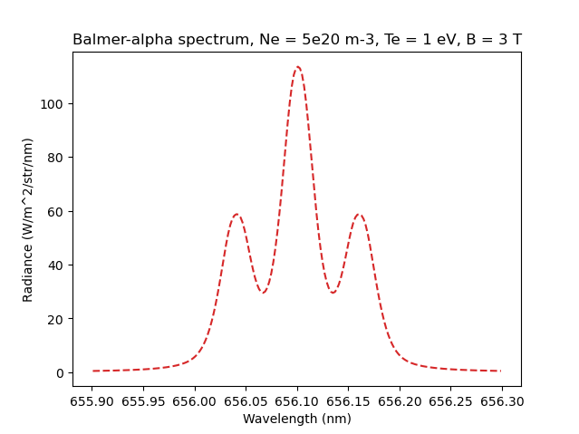
• Zeeman splitting is taken in the form of a simple triplet with a \(\pi\)-component centred at \(\lambda\), \(\sigma^{+}\)-component at \(\frac{hc}{hc/\lambda -\mu B}\) and \(\sigma^{-}\)-component at \(\frac{hc}{hc/\lambda +\mu B}\).

• The convolution of Stark-Zeeman and Doppler profiles is replaced with the weighted sum to speed-up calculations (pseudo-Voigt approximation).

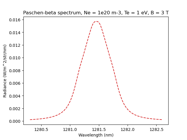
This example calculates Balmer-alpha and Paschen-beta Stark-Zeeman spectral lines for the same parameters of plasma as in Figure 2 in Lomanowski’s paper.

# Copyright 2016-2022 Euratom
# Copyright 2016-2022 United Kingdom Atomic Energy Authority
# Copyright 2016-2022 Centro de Investigaciones Energéticas, Medioambientales y Tecnológicas
#
# Licensed under the EUPL, Version 1.1 or – as soon they will be approved by the
# European Commission - subsequent versions of the EUPL (the "Licence");
# You may not use this work except in compliance with the Licence.
# You may obtain a copy of the Licence at:
#
# https://joinup.ec.europa.eu/software/page/eupl5
#
# Unless required by applicable law or agreed to in writing, software distributed
# under the Licence is distributed on an "AS IS" basis, WITHOUT WARRANTIES OR
# CONDITIONS OF ANY KIND, either express or implied.
#
# See the Licence for the specific language governing permissions and limitations
# under the Licence.

"""
Calculates Balmer-alpha and Paschen-beta Stark-Zeeman spectral lines.

Compare the figures with Figure 2 in B.A. Lomanowski at al, Nucl. Fusion 55 (2015) 123028,
https://iopscience.iop.org/article/10.1088/0029-5515/55/12/123028
"""


# External imports
import matplotlib.pyplot as plt
from raysect.optical import World, Vector3D, Point3D, Ray

# Cherab imports
from cherab.core import Line
from cherab.core.atomic.elements import deuterium
from cherab.core.model import ExcitationLine, StarkBroadenedLine
from cherab.openadas import OpenADAS
from cherab.tools.plasmas.slab import build_constant_slab_plasma


# tunables
ion_density = 2e20
sigma = 0.25

# setup scenegraph
world = World()

# create atomic data source
adas = OpenADAS(permit_extrapolation=True)

# setup the Balmer and Paschen lines
balmer_alpha = Line(deuterium, 0, (3, 2))
paschen_beta = Line(deuterium, 0, (5, 3))

# setup plasma for Balmer-alpha line
plasma_species = [(deuterium, 0, 1.e20, 0.3, Vector3D(0, 0, 0))]
plasma = build_constant_slab_plasma(length=1, width=1, height=1, electron_density=5e20, electron_temperature=1.,
                                    plasma_species=plasma_species, b_field=Vector3D(0, 3., 0), parent=world)
plasma.atomic_data = adas

# add Balmer-alpha line to the plasma
plasma.models = [ExcitationLine(balmer_alpha, lineshape=StarkBroadenedLine)]

# Ray-trace perpendicular to magnetic field and plot the results
r = Ray(origin=Point3D(-5, 0, 0), direction=Vector3D(1, 0, 0),
        min_wavelength=655.9, max_wavelength=656.3, bins=200)
s = r.trace(world)

plt.figure()
plt.plot(s.wavelengths, s.samples, ls='--', color='C3')
plt.xlabel('Wavelength (nm)')
plt.ylabel('Radiance (W/m^2/str/nm)')
plt.title('Balmer-alpha spectrum, Ne = 5e20 m-3, Te = 1 eV, B = 3 T')

plasma.parent = None

# setup plasma for Paschen-beta line
plasma_species = [(deuterium, 0, 1.e20, 0.3, Vector3D(0, 0, 0))]
plasma = build_constant_slab_plasma(length=1, width=1, height=1, electron_density=1e20, electron_temperature=1.,
                                    plasma_species=plasma_species, b_field=Vector3D(0, 3., 0), parent=world)
plasma.atomic_data = adas

# add Paschen-beta line to the plasma
plasma.models = [ExcitationLine(paschen_beta, lineshape=StarkBroadenedLine)]

# Ray-trace perpendicular to magnetic field and plot the results
r = Ray(origin=Point3D(-5, 0, 0), direction=Vector3D(1, 0, 0),
        min_wavelength=1280.3, max_wavelength=1282.6, bins=200)
s = r.trace(world)

plt.figure()
plt.plot(s.wavelengths, s.samples, ls='--', color='C3')
plt.xlabel('Wavelength (nm)')
plt.ylabel('Radiance (W/m^2/str/nm)')
plt.title('Paschen-beta spectrum, Ne = 1e20 m-3, Te = 1 eV, B = 3 T')

plt.show()

Caption: The Stark-Zeeman structure of the Balmer-alpha line.

Caption: The Stark-Zeeman structure of the Paschen-beta line.